Formatting spreadsheet cells
Normally, for the purpose of a presentation, it may be necessary to increase considerably the size of the font as well as matching it to the style used in the presentation.
The fastest and most flexible way to format the embedded spreadsheet is to make use of styles. When working on an embedded spreadsheet, you can access the cell styles created in Calc and use them. However, the best approach is to create specific cell styles for presentation spreadsheets, as the Calc cell styles are likely to be unsuitable when working within Impress.
To apply a style (or indeed manual formatting of the cell attributes) to a cell or group of cells simultaneously, first select the range to which the changes will apply. A range consists of one or more cells, normally forming a rectagular area. A selected range consisting of more than one cell can be recognized easily because all its cells except the active one have a black background. To select a multiple-cell range:
- Click on the first cell belonging to the range (either the left top cell or the right bottom cell of the rectangular area).
- Keep the left mouse button pressed and move the mouse to the opposite corner of the rectangular area which will form the selected range.
- Release the mouse button.
To add further cells to the selection, hold down the Control key and repeat the steps 1 to 3 above.
 | You can also click on the first cell in the range, hold down the Shift key, and click in the cell in the opposite corner. Refer to Chapter 5 (Getting Started with Calc) in the Getting Started book for further information on selecting ranges of cells.
|
Some shortcuts are very useful to speed up the selection:
- To select the whole visible sheet, click at the intersection between the rows indexes and the column indexes, or press Control+A.
- To select a column, click on the column index at the top of the spreadsheet.
- To select a row, click on the row index on the left hand side of the spreadsheet.
Once the range is selected, you can modify the formatting, such as font size, alignment (including vertical alignment), font color, number formats, borders, background and so on. To access these settings, choose Format > Cells from the main menu bar (or right-click and choose Format Cells from the pop-up menu). This command opens the dialog box shown below.
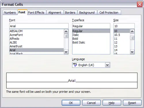
The Format Cells dialog box consists of 7 pages
If the text does not fit the width of the cell, you can increase the width by hovering the mouse over the line separating two columns and, when the mouse cursor changes shape, clicking the left button and dragging the separating line to the new position. A similar procedure can be used to modify the height of a cell (or group of cells).
To insert rows and columns in a spreadsheet, use the Format menu or right-click on the row and column headers and select the appropriate option from the pop‑up menu. To merge multiple cells, select the cells to be merged and select Format > Merge cells from the main menu bar. To de-merge a group of cells, select the group and again Format > Merge Cells (which will now have a checkmark next to it).
When you are satisfied with the formatting and the appearance of the table, exit the edit mode by clicking outside the spreadsheet area. Note that Impress will display exactly the section of the spreadsheet which was on the screen before leaving the edit mode. This allows you to hide additional data from the view, but it may cause the apparent loss of rows and columns. Therefore, take care that the desired part of the spreadsheet is showing on the screen before leaving the edit mode.